3  Elements of Financial Modeling

“Truth … is much too complicated to allow anything but approximations” - John von Neumann

3.1 Chapter Overview

What is a financial model? What are they for? We explore key attributes of models, discuss different approaches and their trade-offs, and get into some philosophy about what models are and how they capture important dynamics about the world.

3.2 What is a Model?

A model is a simplified representation of reality designed to help us understand, analyze, and make predictions about complex systems. In finance, models distill the intricate web of market behaviors, economic factors, and financial instruments into tractable mathematical and computational components. We build models for a variety of reasons, listed in Table 3.1.

Table 3.1: The REDCAPE model use framework, from “The Model Thinker” by Scott Page.

Use	Description
Reason	To identify conditions and deduce logical implications.
Explain	To provide (testable) explanations for empirical phenomena.
Design	To choose features of institutions, policies, and rules.
Communicate	To relate knowledge and understandings.
Act	To guide policy choices and strategic actions.
Predict	To make numerical and categorical predictions of future and unknown phenomena.
Explore	To investigate possibilities and hypotheticals.

For example, say we want to simulate returns for stocks in our retirement portfolio. It would be impossible to build a model capturing all the individual people working jobs and making decisions, weather events damaging property, political machinations, etc. Instead, we try to capture certain fundamental characteristics. It’s common, for instance, to model equity returns as cumulative pluses and minuses from random movements where those movements have certain theoretical or historical characteristics.

Whether we’re using this model of equity returns to estimate available retirement income or replicate an exotic option price, a key aspect of the model is the assumptions used therein. For the retirement income scenario, we might assume a healthy 8% return on stocks and conclude that such a return will be sufficient to retire at age 53. Alternatively, we may assume that future returns follow a stochastic path with a certain distribution of volatility and drift. These two assumption sets produce output—results from our model that must be inspected, questioned, and understood in the context of the “small world” of the model’s mechanistic workings. To be effective practitioners, we must be able to contextualize “small world” results within the “large world” that exists around us.

3.2.1 Small World vs. Large World

The distinction between the modeled “small world” and the real-life “large world” is fundamental to understanding model limitations:

• Small World: The constrained, well-defined environment within your model where all rules and relationships are explicitly specified.
• Large World: The complex, real-world environment where your model must operate, including factors not captured in your assumptions.

Say our model discounts a fixed set of future cashflows using the current US Treasury rate curve. If I run the model today, then re-run it tomorrow with the same future cashflows and the present value has increased by 5%, I might ask: “why has the result changed so much in such a short period?”

In the “small,” mechanistic world of the model, I can see that discount rates have fallen substantially. The small world answer: inputs changed, producing a mechanical change in output. The large world answer: perhaps the Federal Reserve lowered the Federal Funds Rate to prevent the economy from entering a deflationary recession.

We can’t completely explain the relation between our model and the real world (otherwise we could capture that relationship in the model!). An effective practitioner always tries to look up from the immediate work and take stock of how the world at large is or is not reflected in the model.

TipFinancial Modeling Pro Tip

When a model output swings materially between runs, first check the Small World mechanics (e.g., input rates changed) before hypothesizing Large World causes (e.g., policy shifts). Then reconcile both views to avoid over- or under-reacting.

3.3 What is a Financial Model?

Financial models are those used extensively to ascertain better understanding of complex contracts, perform scenario analysis, and inform market participants’ decisions related to perceived value (and therefore price). It can’t be quantified directly, but it is likely not an exaggeration that many billions of dollars transact each day as a result of decisions made from the output of financial models.

Most financial models can be characterized with a focus on the first or both of:

1. Attempting to project patterns of cashflows or obligations at future timepoints
2. Reducing the projected obligations into a current value

Examples of this:

• Projecting a retiree’s savings through time (1), and determining how much they should be saving today for their retirement goal (2)

• Projecting the obligation of an exotic option across different potential paths (1), and determining the premium for that option (2)

• Determining a range of outcomes (1) for risk modeling purposes, and translating those outcomes into a risk or capitalization level (2)

Models are sometimes taken a step further, such as transforming the underlying economic view into an accounting or regulatory view (such as representing associated debits and credits, capital requirements, or associated intangible, capitalized balances). In other words, many models go further than simply modeling anticipated cashflows by building representations of entities (companies or portfolios) which are associated with the cashflows.

3.3.1 Difference from Data Science

We should also distinguish a financial model from a purely statistical model, where inputs and outputs are often known and the intention is to estimate relationships between variables (e.g., linear regression). That said, a financial model may have statistical components, and many aspects of modeling are shared between the two. In this book, we focus on the practice of financial modeling in the ways that it is distinct from statistics and data science. To delineate the practices:

• Statistics, or Statistical Modeling is the practice of applying procedures and probabilistic reasoning to data in order to determine relationships between things or to predict outcomes.
• Data Science includes statistical modeling but also incorporates the art and science of good data hygiene, data pipelines and pre-processing, and more programming than a pure statistician usually uses.

Financial Modeling is similar in the goal of modeling complex relationships or making predictions (a modeled price of an asset is simply a prediction of what its value is), however, it differs from data science in a few ways:

• Financial modeling often encodes theory-driven structures and constraints, then calibrates parameters to data, rather than inferring all relationships purely from data.
• Financial modeling generally contains more unique ‘objects’ than a statistical model. The latter may have derived numerical relationships between data, however a financial model would have things like the concept of a company or portfolio, or sets of individually identifiable assets, or distinct actors in a system.
• Financial modeling often involves a lot more simulation and hypothecating, while data science is focused on drawing conclusions from what data has already been observed.

Nonetheless, there is substantial overlap in practice. For example, the assumption in a financial model (volatility, economic conditions, etc.) may be derived statistically from observed data. Given the overlap in topics, statistical content is sometimes covered in this book (including a from-the-ground-up view of modern Bayesian approaches in Chapter 14).

3.4 Key Considerations for a Model

When creating a model, whether a data model, a conceptual model, or any other type, certain key considerations are generally important to include to ensure it is effective and useful. Some essential considerations include:

Consideration	Description
Objective	Clearly define what the model aims to achieve.
Boundaries	Specify the limits and constraints of the model to avoid scope creep.
Variables	Identify and define all variables involved in the model.
Parameters	Include constants or coefficients that influence the variables.
Dependencies	Describe how variables interact with each other.
Relationships	Detail the connections between different components of the model.
Inputs	Specify the data or resources required for the model to function.
Outputs	Define what results or predictions the model produces.
Underlying Assumptions	Document any assumptions made during the model’s development to clarify its limitations and validity.
Validation Criteria	Outline how the model’s accuracy and reliability are tested.
Performance Metrics	Define the metrics used to evaluate the model’s performance.
Scalability	Ensure the model can handle increased data or complexity if needed.
Adaptability	Allow for adjustments or updates as new information or requirements arise.
Documentation	Provide comprehensive documentation explaining how the model works, including algorithms, data sources, and methods.
Transparency	Make the model’s workings understandable to stakeholders or users.
User Interface	Design an intuitive interface if the model is interactive.
Ease of Use	Ensure that the model is user-friendly and accessible to its intended audience.
Ethics	Address any ethical concerns related to the model’s application or impact.
Regulations	Ensure compliance with relevant laws and regulations.

Including these attributes helps create a robust, reliable, and practical model that effectively serves its intended purpose.

3.5 Predictive versus Explanatory Models

Given a set of inputs, our model generates an output and we’re generally interested in its accuracy. The model need not have a realistic mechanism for how the world works. We may be primarily interested in accurately calculating an output value without the model having any scientific, explanatory power of how different parts of the real-world system interact.

3.5.1 A Historical Example

A historical parallel can be found in the shift from the Ptolemaic to the Copernican model of the solar system. While the Ptolemaic model was predictively accurate for its time, the Copernican model offered a more fundamentally correct explanation of the underlying mechanics¹.

The existing Ptolemaic model used a geocentric view of the solar system in which the planets and sun orbited the Earth in perfect circles with an epicycle used to explain retrograde motion (as seen in Figure 3.1). Retrograde motion is the term used to describe the apparent, temporarily reversed motion of a planet as viewed from Earth when the Earth is overtaking the other planet in orbit around the sun. Despite a fundamentally flawed underlying theory, the geocentric model was accurate enough to match the observational data for the position of the planets in the sky.

Figure 3.1: In the Ptolemaic solar model, the retrograde motion of the planets was explained by adding an epicycle to the circular orbit around the earth.

Famously, Copernicus came along and said that the sun, not the Earth, should be at the center (a heliocentric model). Earth revolves around the sun! Today, we know this to be a much better description of reality than one in which the Earth arrogantly sits at the center of the universe. However, the model was actually slightly less accurate in predicting the apparent position of the planets (to the limits of observational precision at the time)! Why would this be?

First, the Copernican proposal still used perfectly circular orbits with an epicycle adjustment, which we know today to be inaccurate (versus an elliptical orbit consistent with the theory of gravity). Despite being more scientifically correct, it was still not the complete picture.

Second, the geocentric model was already very accurate because it was essentially a Taylor series approximation which described, to sufficient observational accuracy, the apparent position of the planet relative to the Earth. The heliocentric model was effectively a re-parameterization of the orbital approximation.

Third, we have considered a limited criteria for which we are evaluating the model for accuracy, namely apparent position of the planets. It’s not until we contemplate other observational data that the Copernican model would demonstrate greater modeling accuracy: apparent brightness of the planets as they undergo retrograde motion and angular relationship of the planets to the sun.

For modelers today, this demonstrates a few things to keep in mind:

1. Predictive models need not have a scientific, causal structure to make accurate predictions.
2. It is difficult to capture the complete scientific inter-relationships of a system and much care and thought needs to be given in what aspects are included in our model.
3. We should look at, or seek out, additional data that is related to our model because we may accurately overfit to one outcome while achieving an increasingly poor fit to other related variables.

Striving to better understand the world is a good thing to do but trying to include more components into the model is not always going to advance a given goal.

3.5.2 Examples in the Financial Context

3.5.2.1 Home Prices

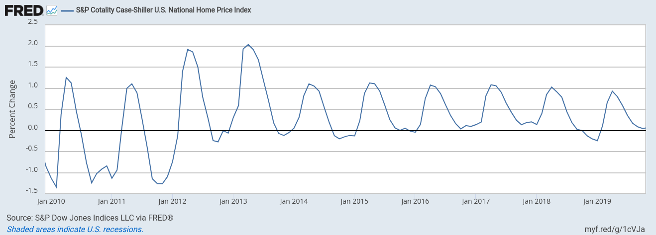
American home prices exhibit strong seasonality and peak around April each year. We may find that a simple oscillating term captures price variability better than imperfectly modeling the true market dynamics: supply and demand curves varying by personal factors (job bonus timing, school calendars), local factors (new homes built, company relocation), and national factors (monetary policy, tax incentives for home-ownership). A simple sinusoidal periodic component could predict this stable pattern well. One could spend months building a more scientific model and not achieve as good a fit, even though the latter tries to be more conceptually accurate.

Figure 3.2: House prices (seasonally unadjusted) often peak around April each year. A simple seasonal component can capture much of this variation without modeling full market microstructure, for example \(p_t = \alpha + \beta \sin(2\pi t/12 + \phi) + \varepsilon_t\), where t is in months.

3.5.2.2 Replicating Portfolio

Another financial modeling example: in attempting to value a portfolio of insurance contracts, a replicating portfolio of hypothetical assets is sometimes constructed² to match a block of complex insurance contracts. The point is to create a basket of assets that can be valued more quickly (minutes to hours) in response to changing market conditions than it would take to run the actuarial model (hours to days). The basket of assets has no ability to explain why the projected cashflows are what they are—but retains strong predictive accuracy.

3.5.3 Predictive vs Explanatory Models in Practice

Section 32.5 describes practical considerations for evaluating models in both predictive and explanatory contexts.

3.6 Types of Models

Different modeling approaches come with their own trade-offs:

Model Type	Description	Examples	Trade-offs	Assumptions
Statistical Models	Use mathematical relationships to describe data.	Linear regression, logistic regression	Simplicity vs. Accuracy: Often simpler and more interpretable but may not capture complex relationships.	Typically rely on assumptions like linearity and normality that may not always hold true.
Machine Learning Models	Learn patterns from data using algorithms.	Decision trees, random forests, neural networks	Complexity vs. Interpretability: Capture complex patterns but are often less interpretable. Overfitting: Risk of overfitting, requiring careful validation and tuning. Data Requirements: Require large datasets.	Performance can degrade with limited or noisy data.
Probabilistic Models	Use probability distributions to model uncertainty and relationships.	Bayesian networks, probabilistic graphical models	Flexibility vs. Computational Complexity: Handle uncertainty and complex relationships but require sophisticated computations.	May require assumptions about the nature of probability distributions and dependencies.
Simulation Models	Use computational models to simulate complex systems or scenarios.	Monte Carlo simulations, agent-based models	Accuracy vs. Computational Expense: Can be computationally expensive and time-consuming. Detail vs. Generalization: High-fidelity simulations may be overkill for simpler problems.	May require simplifications or assumptions for computational feasibility.
Theoretical Models	Based on theoretical principles to explain phenomena.	Economic models, physical models	Precision vs. Practicality: Provide foundational understanding but may rely on idealizations. Applicability: Highly accurate in specific contexts but less so in broader situations.	Often rely on idealizations or simplifications.
Empirical Models	Use historical data to predict future outcomes.	Time series forecasting, econometric models	Data Dependence vs. Predictive Power: Rely heavily on historical data and may not perform well if patterns change. Context Sensitivity: Accurate for specific data but may not generalize well.	Performance is heavily dependent on the quality and relevance of historical data.
Hybrid Models	Combine different modeling approaches to leverage their strengths.	Combining statistical and machine learning approaches	Complexity vs. Versatility: Aim to leverage strengths of different approaches but can be complex to design. Integration Challenges: May present challenges in integration and consistency.	May inherit assumptions from combined models.

Summary of Common Trade-offs:

• Complexity vs. Simplicity: More complex models can capture more nuanced details but are harder to understand and manage.
• Accuracy vs. Interpretability: High-accuracy models may be less interpretable, making it harder to understand their decision-making process.
• Data Requirements: Some models require large amounts of data or very specific types of data, which can be a limitation in practice.
• Computational Resources: More sophisticated models or simulations can require significant computational power, which may not always be feasible.

Understanding these trade-offs helps select the most appropriate modeling approach for your specific problem and available resources.

---

1. Prof. Richard Fitzpatrick has excellent coverage of the associated mathematics and implications in “A Modern Almagest”: https://farside.ph.utexas.edu/books/Syntaxis/Almagest/Almagest.html

2. See, e.g., SOA Investment Symposium March 2010. Replicating Portfolios in the Insurance Industry (Curt Burmeister Mike Dorsel Patricia Matson)