@time exp(rand()) 0.000000 seconds2.388704053480481“Simple things should be simple, complex things should be possible.” - Alan Kay (1970s)
Abstraction matters as a technique in its own right. This chapter focuses on code organization, interfaces, and reusable design patterns.
In programming and modeling, as in mathematics, abstraction permits the definition of interchangeable components and patterns that can be reused. Abstraction is a selective ignorance - focusing on the aspects of the problem that are relevant, and ignoring the others. The last two chapters described what we might call “micro-level” abstractions: specific functions and types.
In this chapter, we zoom out and examine some principles that guide good model development, manifesting in architectural concerns such as how different parts of the code are organized, what parts of the program are considered ‘public’ versus ‘private’, and patterns themselves.
Chapter 5 described a number of tools that we can utilize as interfaces within our model. We use these tools that are provided by our programming language in service of the conceptual abstraction described above.
Table 8.1 lists some principles that arise when developing a particular abstraction. Not all abstractions serve all of these purposes but generally fit one or more of them. These principles provide guidance for creating abstractions that are modular, reusable, and maintainable. By following these principles, developers can create financial models that are easier to understand, extend, and adapt to changing requirements.
| Principle | What | Why | Example |
|---|---|---|---|
| Separation of Concerns | Divide the system into distinct parts, each addressing a separate concern. | Promote modularity and reduce coupling between components. | Separating data retrieval, data processing, and output generation steps in a process. |
| Encapsulation | Hide the internal details of a component and expose only a clean, well-defined set of functionality (interface). | Prevent other parts of the program from modifying internal data, making the system easier to understand and maintain. | Defining a type or module with well-defined behavior and responsibility. |
| Composability | Design simple components that can be combined to create more complex behaviors, rather than a single component that attempts to handle all behavior. | Promote reuse and allow for the components to be combined creatively. | Separate details about economic conditions into different types than contracts/instruments. |
| Generalization | Identify common patterns and create generic components that can be specialized as needed. Often this means identifying common behaviors that arise repeatedly in a model. | Avoid duplication and make the system more expressive and extensible. | Defining a generic Instrument type that can be specialized for different asset classes. |
This strategy groups together components within a model that behave similarly. So, in our example, bonds and interest-rate swaps fundamentally share many characteristics and are used in very similar ways within a model. Therefore, it might make sense to group them together when developing a model.
It may be that components of the model require sufficient expertise that different persons or groups are involved in the development. This may warrant separating a model’s design so that different groups can focus on more specific aspects, regardless of similarities among components. For example, at a higher vertical level of abstraction, financial derivatives may fall under a similar grouping, but sufficient differences exist for equity, credit, or foreign exchange derivatives that the model should separate those three asset classes for development purposes.
For some model design goals, it may be warranted to bundle together more functionality instead of allowing users to compose functionality that comes from different packages. For example, perhaps a certain visualization of model results is particularly useful, not easy to create from scratch, and it is widely desired to see the model output visualized that way. Instead of relying on the user to install a separate visualization package and develop the visualization themselves, it could make sense to bundle visualization functionality with a model that is otherwise unconcerned with graphical capabilities.
In general, loosely coupled systems are preferred—you want to pick and choose which components you use while ensuring they work well together.
Interfaces are the boundaries between different encapsulated abstractions. The user-facing interface is what users of a package or model must actually think about—separate from the intermediate variables, logic, and complexity hidden within.
When looking up a ticker for a market quote, one need not be mindful of the underlying realtime databases, networking, rendering text to the screen, memory management, etc. The interface is “put in symbol, get out number”. By design, there are multiple layers of interfaces and abstractions used under the hood, but the financial modeler need only be actively concerned about the points that he or she comes in contact with, not the entire chain of complexity.
For a financial model, there might be interfaces for bonds or interest rate swaps, and separate interfaces for calculating risk metrics or visualizing results. Good design separates visualization concerns from contract mechanics and other domain logic. Open-source ecosystems (for visualization, data frames, file I/O, statistics, etc.) make these boundaries easier to see; the hard part is drawing similar boundaries inside your financial model.
However, it’s often difficult to find where to draw lines within financial models. For example, should bonds and interest-rate swaps be in separate packages? Or both part of a broader fixed income package? This is where much of the art and domain expertise of the financial professional comes to bear in modeling. There would be no way for a pure software engineer to think about the right design for the system without understanding how underlying components share similarities or differences and how those components interact.
A well-designed interface should follow these principles:
As a case study, we will look at the FinanceModels.jl and related packages to discuss some of the background and design choices that went into the functionality. This suite was written by one of the authors and is publicly available as a set of installable Julia packages.
In actuarial work, you constantly work with interest rate and bond yield curves—determining forward rates, estimating the shape of future curves, or discounting cashflows to estimate a present value. Determining things like “given a par yield curve, what’s the implied discount factor for a cashflow at time 10” or “what is the 10 year BBB public corporate rate implied by the current curve in five years’ time” is cumbersome at best in a spreadsheet.
For example, to determine the answer to the first one (“a discount factor for time 10”) actually requires quite a bit of detail and assumption to derive:
0.05 for time 10, is it quoted as a continuously compounded rate or as an annual effective rate? Is that a par rate, a zero-coupon bond (spot) rate, or a one-year-forward rate from time 10?This is exactly the kind of complexity we want to hide when the goal is simply to value a stream of riskless life insurance payments, which might look like this:
  risk_free_rates = [0.05, 0.055, 0.06]      # example par yields
  tenors = [1.0, 5.0, 10.0]                  # years
  yield_curve = Yields.Par(risk_free_rates, tenors)

  cashflow_vector = [1_000_000.0, 3_000_000.0, 1_000.0]
  present_value(yield_curve, cashflow_vector)
The variable and function names make the purpose and steps clear. Now imagine doing this in a spreadsheet: bootstrapping, interpolation, and discounting before you even get to the present value you actually wanted. What can be five lines of code (with the right abstractions) would take hundreds of cells in a spreadsheet. Abstractions like these are productivity multipliers for financial modelers.
Two main abstractions emerged in the early versions.
Utilizing the benefit of the type system, it was decided that it would be most useful to represent rates not as simple floating point numbers (e.g. 0.05) but instead with dedicated types to distinguish between rate conventions. The abstract type CompoundingFrequency had two subtypes: Continuous and Periodic so that a 5% rate compounded continuously versus an effective per period rate would be distinguished via Continuous(0.05) versus Periodic(0.05,1). The two could be converted between by extending the built-in Base.convert function.
This was useful because once rates were converted into Rates within the ecosystem, that data contained within itself characteristics that could distinguish how downstream functionality should treat the rates.
At first, only bootstrapping was supported as a method to construct curve objects. This required that there was only one rate given per time period (no noisy data) and only supported linear, quadratic, and cubic splines.
Further, there was a specific constructor for different common types of instruments. From the old documentation:
Yields.Zero(rates,maturities)using a vector of zero, or spot, ratesYields.Forward(rates,maturities)using a vector of one-period forward ratesYields.Constant(rate)takes a single constant rate for all timesYields.Par(rates,maturities)takes a series of yields for securities priced at par. Assumes that maturities <= 1 year do not pay coupons and that after one year, pays coupons with frequency equal to the CompoundingFrequency of the corresponding rate.Yields.CMT(rates,maturities)takes the most commonly presented rate data (e.g. Treasury.gov) and bootstraps the curve given the combination of bills and bonds.Yields.OIS(rates,maturities)takes the most commonly presented rate data for overnight swaps and bootstraps the curve.
This covered a lot of lightweight use-cases, but made a lot of implicit assumptions about how the given rates should be interpreted.
Several insights led to a more flexible interface in later versions.
First, realizing that yield curves were just a particular kind of model - one that used interest rates to discount cashflows. But you can have different kinds of models - such as Black-Scholes option valuation or a Monte Carlo valuation approach. Likewise, the cashflows need not simply be a vector of floating point values, and instead it could be the representation of a generic financial contract. As long as the model knew how to value it, an appropriate present value could be derived.
Where previously it was:
present_value(yield_curve,cashflow_vector)Now, it was
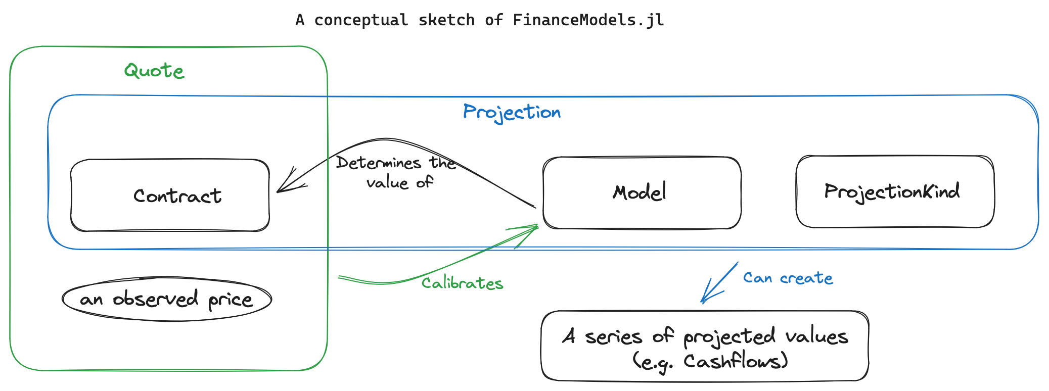
present_value(model,contract)Second, that a model was simply some generic box that had been “fit” to previously observed prices for similar types of contracts we would be trying to value in the model. The combination of a contract and a price constituted a “quote” and with multiple quotes a model could be fit using various algorithms.
With these changes, the package that was originally called Yields.jl was renamed to FinanceModels.jl. The updated code from the earlier example now would be implemented like this:
using FinanceModels
risk_free_rates = [0.05, 0.055, 0.06]
tenors = [1.0, 5.0, 10.0]
quotes = ParYield.(risk_free_rates, tenors)

model = fit(Spline.Cubic(), quotes, Fit.Bootstrap())

cashflow_vector = [1_000_000.0, 3_000_000.0, 1_000.0]
present_value(model, cashflow_vector)
It’s slightly more verbose, but notice how much more powerful and extensible fit(Spline.Cubic(), quotes, Fit.Bootstrap()) is than Yields.Par(risk_free_rates,tenors). The end result is the same, but now the same package and interface can clearly interchange other options, such as a NelsonSiegelSvensson curve instead of a spline. And the quotes could be a combination of observed bonds of different technical parameters (though still sharing characteristics which make it relevant for the model being constructed).
The same pattern also applies to option valuation, such as this example of vanilla euro options with an assumed constant volatility assumption:
EuroCall are the underlying asset type, strike, and maturity time.
0.15 for the 1-year call (given the quoted price).
0.0541.
With a consistent interface that handles a wide variety of situations, you’re free to expand the model in new directions. The built-in functionality lets you compose pieces together in ways that weren’t possible with the less abstracted design. For example, the equity option example had no parallel when all of the available constructors were Yields.Zero or Yields.Par and would have required a completely from-scratch implementation with newly defined functions.
Further, and critically, the new design allows modelers to create their own models or contracts1 and extend the existing methods rather than needing to create their own: the function signature fit(model,quotes) handles a very wide variety of cases, as does present_value(model,contract).
When you are introducing a new abstraction in a production model, walk through the following quick diagnostic:
Keeping these questions in mind ensures the abstraction remains a tool, not a new source of opacity.
We have talked about transforming data and restructuring logic in order to make the model more effective. We can go even further: we can abstract the process of writing code itself. This subject is a bit advanced, so we are simply going to introduce it because you will likely find many convenient instances of it as a user even if you never need to implement it yourself.
Homoiconicity refers to the property of a programming language where the language’s code can be represented and manipulated as a data structure in the language itself. Think of a recipe. You can follow the recipe’s instructions to bake a cake — that’s like executing code. But you could also treat the recipe itself as data to be analyzed or transformed: you could write a program to scan thousands of recipes, find every instance of “sugar,” and reduce the quantity by 25%. This is the essence of homoiconicity: the same representation serves both as executable instructions and as data that can be inspected or transformed.
In a homoiconic language like Julia, the code is data and can be treated as such. This enables powerful metaprogramming (i.e. code that writes other code) capabilities, where code can generate or transform code during macro expansion (before runtime), producing expressions that are then compiled.
Macros are a metaprogramming feature that leverage homoiconicity in Julia. They allow the programmer to write code that generates or manipulates other code at compile-time. Macros take code as input, transform it based on certain rules or patterns, and return the modified code which then gets compiled.
For example, a built-in macro is @time which will measure the elapsed runtime for a piece of code2.
@time exp(rand())Will effectively expand to:
t0 = time_ns()
value = exp(rand())
t1 = time_ns()
println("elapsed time: ", (t1-t0)/1e9, " seconds")
value
Here it is when we run it:
@time exp(rand()) 0.000000 seconds2.388704053480481In the context of financial modeling, macros can be used to simplify repetitive or complex code patterns, enforce certain conventions or constraints, or generate code based on data or configuration.
Here are a few potential use cases of macros in financial modeling. Again, these are more advanced use-cases but knowing that these paths exist may benefit your work in the future.
Defining custom DSLs (Domain-Specific Languages): Macros can be used to create expressive and concise DSLs tailored to financial modeling. For example, a macro could allow defining financial contracts using syntax closer to the domain language, which then gets expanded into the underlying implementation code.
Automating boilerplate code: Macros can help reduce code duplication by generating common patterns or boilerplate code. This can include generating accessor functions3, constructors, or serialization logic based on type definitions.
Enforcing conventions and constraints: Macros can be used to enforce coding conventions, such as naming rules or type checks, by automatically transforming code that doesn’t adhere to the conventions. They can also be used to add runtime assertions or checks based on certain conditions.
Optimizing performance: Macros can be used to perform code optimizations at compile-time. For example, a macro could unroll loops, inline functions, or specialize generic code based on specific types or parameters, resulting in more efficient runtime code.
Generating code from data: Macros can be used to generate code based on external data or configuration files. For example, a macro could read a specification file and generate the corresponding financial contract types and functions.
present_value(model, contract)) so that new instruments or calibration routines can be composed without editing core logic.And projections, which is handled by defining a ProjectionKind, such as a cashflow or accounting basis. This topic is covered in more detail in the FinanceModels.jl documentation.↩︎
@time is a simple, built-in macro. For true benchmarking purposes, see Section 24.4.↩︎
Accessor functions are useful when working with nested data structures. For example, if you have a struct within a struct and want to conveniently access an inner struct’s field.↩︎